Deploying a Machine Learning Model into Production on VMware with H2O, Apache Spark and GPUs

In an earlier VMware blog article and demo on machine learning, we used the H2O Driverless AI tool, deployed on VMware vSphere-based VMs, for feature engineering, choosing and training a machine learning model and finally for creation of a deployable ML pipeline. A big advantage of using this H2O Driverless AI tool in virtual machine form on VMware is the ability to have multiple separate activities going on at the same time on common infrastructure, such as multiple training phases, or a mix of concurrent training and inference using GPU-enabled and non GPU-enabled VMs. The details of setting up your VMs for GPUs are given in a series of posts here. We tested different versions of the H2O Driverless AI tool and different VMs on different host servers with and without GPUs for execution of the ML pipeline in the work described here. Many ML algorithms used in H2O are GPU accelerated today. This article describes the various options for production deployment of ML pipelines using H2O’s tools, the JVM and the Apache Spark platform.

Once we complete our automated training/model creation in the H2O Driverless AI environment, we have a trained model with a certain prediction accuracy score, contained in a pipeline for execution. “Pipelines” are commonly used in machine learning practice as a mechanism for carrying out several actions on a data set, including model-based prediction or classification. The deliverable, or unit of deployment is therefore the pipeline itself. Below we see the user interface to the H2O Driverless AI tool as it appears at the end of a model training process. That training was conducted with a dataset made up of 24,000 records of credit card payment history data.

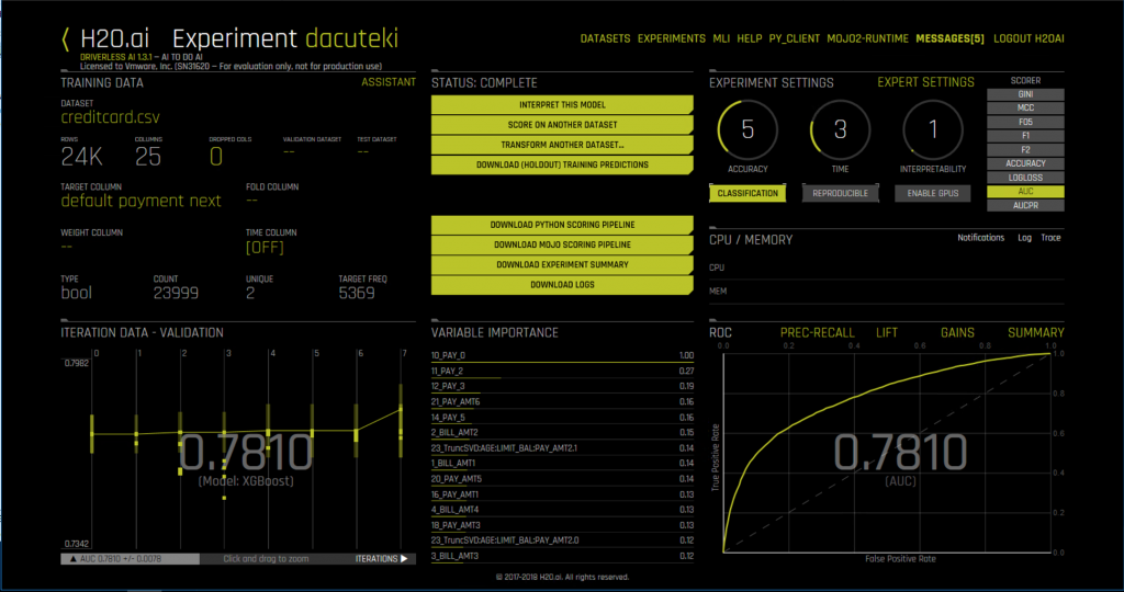
The details of this interface are given here. We won’t go into those UI details further in this article. Suffice it to say that this is a sophisticated tool for the data scientist that helps with many parts of that person’s work, such as data visualization, feature engineering, feature importance, model choice and model parameter tuning. The model chosen by the tool in the experiment above, seen in the “Iteration Data” section on the lower left, is an XGBoost one, a leading method in the Gradient Boosting Machines field, that is well known for dealing well with tabular data, such as we have here. The Driverless AI tool is designed for supervised learning on datasets such as this.

A data scientist may use the “Area Under the Curve” or AUC (seen on the right in the H2O Driverless AI tool ) to judge the accuracy of the model. The model training phase is done iteratively by the data scientist to get the best possible accuracy of the model, based on the separate training and testing datasets. This article does not focus on achieving higher model accuracy, but instead assumes accuracy is satisfactory and we now take the next step – we deploy a pipeline, produced by the Driverless AI tool, into a production cluster to do inference. In this case, inference involves prediction of the likelihood of a default on a credit card payment. You should consider this deployment scenario as an example of how a business application, such as one used in a financial institution, could use the ML pipeline’s functionality. You can think of the ML pipeline as a software component that is called many times by one or more business applications  – but using different test/production data. This could be part of a credit card risk analysis or other analysis on a set of customer data, for example. The pipeline and trained model will need to be re-trained on fresh training data and re-deployed to production on a regular schedule, so that it does not drift in its accuracy over time.

We use the Java runtime (JVM) and an Apache Spark cluster as choices for the robust platform supporting production deployment of the model. You could use either of these in production – or choose other platforms, such as PySparkling or MLleap, too.

Having run the training phase of ML model development, we now use the “Download MOJO Scoring Pipeline” menu item from the center menu of the Driverless AI summary screen to retrieve the trained model from the tool, encapsulated in a pipeline (itself a file). We will refer to both the trained model and the pipeline collectively as the “pipeline” here. The acronym “MOJO” in the context of H2O’s products means “Model Optimized Java Object”. This is a more compact and performant deliverable for a model and pipeline than the earlier Plain Old Java Object (POJO) form, which had a tendency to be very large, for certain model and data types. POJOs are still available, but a MOJO is seen as the optimal deliverable to be deployed of the two. A MOJO pipeline is invoked by a consuming class/process in the same way as a POJO would be. We will see two examples of that usage below. The term “Scoring” refers here to production time use of an ML trained model for inference (prediction) on new data, that it has not seen before.

NOTE: Before you train your model in a Driverless AI “experiment”, the following variable must be set to “true” in the Driverless AI configuration file located at /etc/dai/config.toml on Linux. The Driverless AI processes must be restarted in order for that “Download MOJO Scoring Pipeline” setting to work.

make_mojo_scoring_pipeline = true

This setting is required in order for Driverless AI to allow the “Download MJO Scoring Pipeline” feature to work. Before making that change, we first stop the Driverless AI processes using the command

systemctl stop dai

Once we have made the above config.toml file change, we restart the Driverless AI processes using

systemctl start dai

Below we see the user choosing a destination for the downloaded MOJO file.

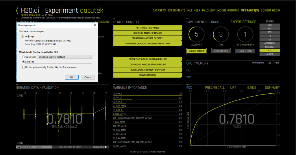
This output data comes down to our workstation as a “.zip” file that we unzip to retrieve the contained “pipeline.mojo” file – the latter is the key deliverable for production use. You can look at the contents of the downloaded .zip using the command

unzip -l <name of mojo zip file>

Below we see an example of the contents of the downloaded .zip file. You can see the “pipeline.mojo” file that we will be using for deployment later on in this article, along with an example shell script that shows how to run it. The “mojo2-runtime.jar” file is also important here.

NOTE: As we move between different versions of Driverless AI tools and models, in different virtual machines, we need to be cognizant of the consistent versioning of these two files. They must come from the same model training experiment and the same version of the Driverless AI tool. Newer versions of the mojo2-runtime.jar classes can understand and deploy older pipelines, but the reverse is not supported currently.

Virtual Machines with GPUs for Training and without GPUs for Inference

We used different virtual machines in each of the categories above. We wanted to test whether we could

• deploy different versions of Driverless AI and conduct separate model training exercises with them, independently
• deploy the created models interchangeably on a common VM platform, even if created by different versions of Driverless AI
• train a model in a Driverless AI tool that runs on a GPU-enabled VM and then deploy the resulting pipeline in a non-GPU enabled VM.

The last test was designed to show that the more compute-intensive ML training process could exploit the power of a GPU whereas the same GPU power may not be needed for inference on a separate virtual machine. These VMs were hosted on different servers. We tested the inference (or “scoring”)  on a VM where a GPU was not present. We succeeded in proving all three of the above conditions with a set of virtual machines as shown in the VMware vSphere Client management interface below. The vSphere Client is a browser-based interface to a widely-used VMware management server, the vCenter Server, which controls and monitors both physical and virtual machines in a data center.

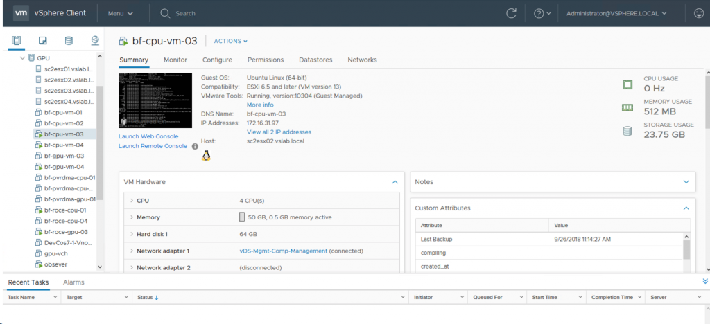
For those who may be new to the vSphere Client tool, the items labeled “sc2esx<nn>.vslab” in the left navigation are four physical host servers in our data center with our collection of virtual machines running on them. These are in use by several people concurrently in our environment. The “bf-cpu-vm-<nn>” objects are virtual machines that are not enabled with GPUs. The “bf-gpu-vm-<nn>” objects are those VMs that have GPUs enabled, using VMware’s Passthrough mode here. For the different choices you can make about GPUs and more technical information on configuring GPUs with virtual machines on VMware, see the articles here. GPUs and machine learning applications have been tested heavily for performance over long periods of time on VMware and you can read more about that performance area here

Production Deployment Choices for a Machine Learning Pipeline

For the purposes of our deployment testing, we used the classic “creditcard.csv” dataset example that comes with the H2O Driverless AI environment. Once we have trained our model and pipeline, we then consider the options for a platform for production deployment. It is widely accepted that Apache Spark is an important platform component for different parts of the Machine Learning pipeline. This is because Spark offers sophisticated ML pipelines and data handling APIs of its own, along with the power of a scale-out cluster where predictions may be done in parallel on separate parts of the data. Another viable option is deploying a process in a JVM, or using the MLleap technology. H2O’s data scientists and engineers have seen all three types of deployment used for production deployment.

Because of previous experience with Apache Spark standalone, and its simplicity of deployment, we chose to use it here, along with some components from the H2O Sparkling Water libraries. Here is an image showing how Spark helps with the model development and deployment phases. As you can see, its functionality is complementary to that of H2O. It is also possible to deploy Spark in a Hadoop/YARN environment, and that is explained in detail in the H2O documentation so we won’t go into it here.

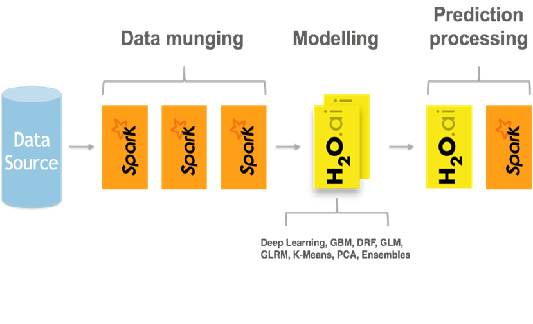
As you can see from the above, Apache Spark, shown in orange, is very useful for the data cleansing/data preparation phase. This is because of its powerful APIs and SQL functionality. Along with feature engineering, this is called “data munging” here. Importantly, Apache Spark is also a deployment time platform for prediction processing, alongside H2O platforms.

There are several options for using H2O and Apache Spark together. These include using H2O’s Sparkling Water, which allows you to run the two platforms together. One style is to design an “external” deployment of H2O Sparkling Water, where the H2O cluster and the Apache Spark cluster are separated, as seen below. That Sparkling Water setup, in practice, is used mainly for training and testing the model. We delve into this subject in more depth in Appendix 2 below.

For “scoring” or the production phase of the model’s lifetime, we wanted to use standalone Apache Spark and the Java virtual machine as the runtime engines, as those are in very popular use for business application support today. In this work, we exploit some of the Sparkling Water libraries that will be loaded into the Apache Spark and Java production runtimes as Jar files.

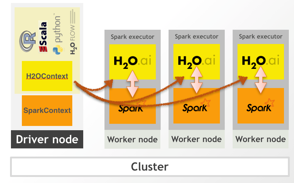
To simplify the approach for production deployment, we use the Apache Spark runtime (standalone) with a small cluster composed of one master and one worker node, initially, to execute our pipeline for prediction. The master and worker can live in the same VM or in separate VMs. We can easily scale up the number of Spark worker/slave nodes in the cluster for a larger deployment.

We need some wrapper code to execute the ML pipeline with a set of test input data and to produce some output prediction data. There is a convenient class for deploying a MOJO pipeline, described in the H2O documentation here, named

org.apache.spark.ml.h2o.models.H2OMOJOPipelineModel

That class is available as a component of the Sparkling Water product – hence we installed that H2O platform also. We used the Sparkling Water 2.4.5 environment described in Appendix 2 for other testing before delivering the pipeline to the production phase. Sparkling Water may also be used in production environments where H2O and Apache Spark APIs and pipelines are required to be used closely together. This was not a requirement in the current work.

Setting the Environment Variables

We set the following environment variables for our Standalone Spark and H2O Sparkling Water environment. In our case the /home/spark-2.4.0-bin-hadoop2.7 directory was where we installed Apache Spark to begin with.

PATH=/home/spark-2.4.0-bin-hadoop2.7/bin:/home/spark-2.4.0-bin-hadoop2.7/sbin:$PATH

SPARK_HOME=/home/spark-2.4.0-bin-hadoop2.7

The SPARK_HOME location was where we installed Apache Spark 2.4.0.

Prerequisites for Sparkling Water

We extended the Sparkling Water system to be compatible with Driverless AI using the instructions given here 

1. Build the Sparkling-Water-Assembly.jar File

This Jar file is needed for an “external” Sparkling Water cluster deployment. This step may be skipped for the current production deployment work. It is included here for completeness and for reference in Appendix 2. We use the command

apt install gradle

to get the “gradlew” build tool into our VM and

gradlew build -x check

to create the file called /home/sparkling-water-2.4.5/assembly/build/libs/sparkling-water-assembly_2.11-2.4.5-all.jar.

That gradlew build process produces the Jar file above that is included on the various command lines used at “spark-shell” and “spark-submit” invocation time.

2.  Download the H2O-extended.jar File

NOTE: This Jar file contains an important class named H2OMOJOPipelineModel that we use for testing and production. Because we wanted to use this class, that provided our essential motivation for working with Sparkling Water here. We also wanted to explore the External Backend deployment of the Sparkling Water setup as described here

You can read more about this in Appendix 2 below. To complete this part of the setup, we followed the instructions in the documentation that required the download of the Extended-H2O.jar file, as follows:-

$SPARKLING-WATER-HOME/bin/get-extended-h2o.sh standalone

NOTE: The parameter supplied to the above shell script would differ for implementations other than Spark standalone, such as those run on Hadoop. Consult the H2O documentation for these situations.

Pre-Production Pipeline Testing

The following testing of the scoring pipeline (i.e. the MOJO) would be done before placing it into a more robust production deployment. Here, we wanted to interact with the pipeline by feeding it some test data and ensuring that it produced the expected results for any inputs. The interactive Spark Shell allowed us to do that.

NOTE: You will need to supply your H2O Driverless AI license file as one of the parameters given with the –jars option.

To run the Spark Shell and test our pipeline, we execute the following command:

spark-shell –jars license.sig,/opt/h2oai/dai/mojo2-runtime.jar,/home/sparkling-water-2.4.5/assembly/build/libs/sparkling-water-assembly_2.11-2.4.5-all.jar –driver-memory 5g –executor-memory 4G –executor-cores 2

This brings up an interactive shell session in Spark, where we can execute Scala commands and scripts. We used Scala for the test scripts executing the model pipeline here. Scala is a native language to Spark, though you may also choose to use Python, Java or the R language if you wish to.

Execute a Test Program for the Pipeline in the Spark Shell

In the running Spark-shell, we can either type in the individual commands below interactively or load a script for execution. In our testing, we used a test.scala script containing the code given below. This full script was then executed when we typed the load command in the shell:

:load test.scala

Here are the contents of that “test.scala” file.

// Testing code for the MOJO Pipeline from a Driverless AI modeling exercise

import spark.implicits._

import org.apache.spark.sql.Dataset

import org.apache.spark.ml.h2o.models.H2OMOJOPipelineModel

import org.apache.spark.h2o._

import org.apache.spark.ml.h2o.models._

val mojo = H2OMOJOPipelineModel.createFromMojo(“file:///<name of the pipeline.mojo file>”)

mojo.setNamedMojoOutputColumns(true)

// Read the test data set in from a file into a Spark DataFrame, df – think of this as similar to a table

val df = spark.read.option(“header”, “true”).csv(“file:///<name of the creditcard.csv file>”)

df.show

// Execute the MOJO pipeline containing the trained model against the test data in the Dataframe df

// using the “transform()” method. Store the results of the scoring in “predictions”

val predictions = mojo.transform(df)

// Select a prediction from the resulting set using its column name, this one is for no default payment

predictions.select(mojo.selectPredictionUDF(“default payment next month.0”)).show

// And the predictions for a payment default occurrence (value =1)

predictions.select(mojo.selectPredictionUDF(“default payment next month.1”)).show

Using the above code in the Spark Shell, we can see our pipeline in action against a number of representative test data sets and ensure that we are happy with the outcome from the model.

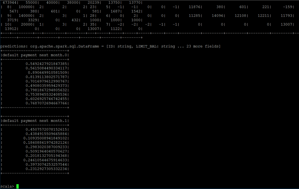
Below is a snapshot of the output from the code. The 20 lines of output in the lowermost two tables, with the title “default payment next month.0” and “default payment next month.1”  show the model’s prediction probability values for the “no default” condition (.0) and the “default is likely” condition (.1) . These values would then be used in the business application logic We ran similar tests with 20,000 test examples to see the performance of the model. It completed prediction for those tests within acceptable times (within 0.25 minutes).

Production Deployment

When we are ready to deliver our pipeline into production, we want to use either (1) a JVM (Java Virtual Machine) or (2) a full Apache Spark cluster as the deployment platform. The latter is composed of a master process and one or more worker/slave processes, for scaling and for cluster robustness against one or more process failures. The size of the Spark cluster, in terms of number of nodes depends on the needs of the workload. This Spark environment could be within a Hadoop cluster and scheduled using YARN. For our purposes here, we used standalone Spark, outside of YARN. Apache Spark and other forms of Spark have been tested extensively in VMware’s performance engineering labs. Here is one of a set of reports on that subject.

1. Deploying the ML Pipeline Using the Java Runtime

You can execute a MOJO pipeline very simply using just the JVM. This is the easiest way to deploy your pipeline. In our example, given the MOJO file created in the DriverlessAI too, in our case the file named “pipeline.mojo” and the appropriate Driverless AI license file and Jar file shown below, we can execute in Java using the command here:

java -Dai.h2o.mojos.runtime.license.file=license.sig -cp /opt/h2oai/dai/mojo2-runtime.jar ai.h2o.mojos.ExecuteMojo pipeline.mojo Inputcreditcard.csv OutputPredictions.csv

This executes the class ai.h2o.mojos.ExecuteMojo using the file “pipeline.mojo” as the pipeline to run, with an input test dataset (Inputcreditcard.csv) and an output file (OutputPredictions.csv). It produces a set of predictions on the “default payment next month” field for the “will default on payment” or “no default” condition.

The output from this command looks like the following:

Mojo load time: 399.000 msec
Time per row: 39 usec (total time: 959.000 msec)

In the output file from this prediction work (the file OutputPredictions.csv in our example), we see two columns, one showing a prediction on probability of a negative condition on a “default payment next month” and the second showing a probability a positive condition for that default. This would then be taken further by the business application. We show the results for just 10 examples – there can of course by a lot more.

default payment next month.0,  default payment next month.1
0.5492427921847385,                  0.4507572078152615
0.5615084490334117,                   0.4384915509665884
0.890649910581509,                    0.10935008941849102

For larger MOJO pipelines and larger datasets, having the prediction logic and the dataset spread over several compute nodes/VMs gives us the ability to do prediction in parallel and therefore increase the speed of execution. Spark’s ability to hold data in memory in a distributed form (using resilient distributed datasets or RDDs) is a big benefit here.

2. Deploying the ML Pipeline on a Standalone Apache Spark Cluster

Before we can execute a job on a Spark cluster, we need to start the key components of the cluster, the Spark master and worker/slave processes. The example used here is a minimal cluster involving one master and one worker process. There can be any number of workers spread across different virtual machines on different host servers. Spark can also be initiated in containers under Kubernetes control and that is shown in a separate publication.

2.1 Start the Spark Cluster

To start the Spark master and worker processes, use the following commands:

$SPARK_HOME/sbin/start-master.sh

and

$SPARK_HOME/sbin/start-slave.sh spark://<IP Address of Master VM>:7077

Once these processes have started, you can use your browser to view the Apache Spark console by going to the URL

http://<IP Address or hostname of Master VM>:8080.

There we see the various components of the Spark environment, such as the applications that are running or completed. By drilling into an application entry, we see the Spark Executors (JVMs) that carry out the work for any one job. We allocated two cores per Executor for this inference job, and Spark allocated two executors per worker virtual machine dynamically.

Here is what we see in the Spark console after executing our job a number of times. The “Completed Applications” section shows the tests we did with the PredictCC program below.

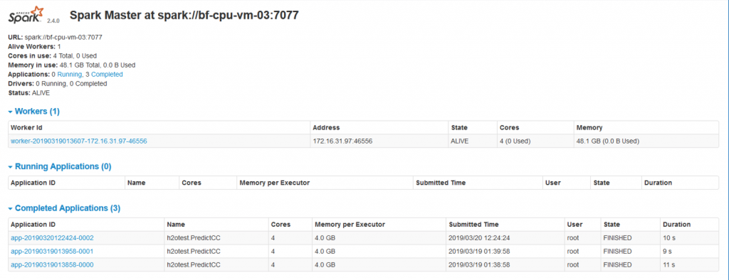
We can have any number of nodes or members of the Spark Worker nodes seen above, depending on our compute resources. This provides us with a Spark cluster that is ready to accept jobs for execution. We use the standard Spark console to view those jobs and their progress.

2.1. Submit a Job to the Spark Master

Before we submit our prediction job, we compile a simple test program that executes the code to test our MOJO pipeline and the model contained in it. In our work, we chose to use the Scala language for this. The program that was used closely resembled the one above we used in the Spark shell, with some small syntactic differences. We compiled this using the “scalac” compiler at version 2.12.8

// PredictCC.scala – uses the pipeline in MOJO form that was created by Driverless AI for Predicting Default

// probability on credit card payment next month.

package h2otest

import org.apache.spark._
import org.apache.spark.SparkContext
import org.apache.spark.sql.SparkSession
import org.apache.spark.sql.Dataset
import org.apache.spark.sql.Row
import org.apache.spark.ml.h2o.models.H2OMOJOPipelineModel
import org.apache.spark.h2o._
import org.apache.spark.ml.h2o.models._
import water.support.SparkContextSupport

object PredictCC {

def main(args: Array[String])

{

val sparkConf = new SparkConf(true)
val sparkContext = new SparkContext(sparkConf)

val spark = SparkSession.builder().appName(“TestH2O”).config(“spark.sql.warehouse.dir”, new String(“/tmp”)).enableHiveSupport().getOrCreate()

//Read in the MOJO pipeline from the file downloaded from Driverless AI

val mojo = H2OMOJOPipelineModel.createFromMojo(“file:///ml_data/justin/tmp/mojo-pipeline/pipeline.mojo”)

mojo.setNamedMojoOutputColumns(true)

// Use the test data to create a DataFrame object

val df = spark.read.option(“header”, “true”).csv(“file:///home/sparkling-water-2.4.5/bin/test-creditcard.csv”)

df.show

// Run the MOJO pipeline on the input data to generate predictions

val predictions = mojo.transform(df)

predictions.show

}

}

Once we have packaged the output .class file from the Scala compiler (scalac) into a suitable Jar file using the command

 jar cvf h2otest.jar h2otest/*

we can then use the  “spark-submit” command in Apache Spark to submit our job to the Spark master node as shown below. This executes the PredictCC program code shown above, with our fixed input and output file names. These fixed file names could be changed to use arg[1] and args[2] for the file names instead for more flexibility.

spark-submit –class h2otest.PredictCC –master spark://172.16.31.97:7077 –driver-memory 5g –executor-memory 4G –executor-cores 2 –jars license.sig,/home/sparkling-water-2.4.5/bin/h2otest.jar,/opt/h2oai/dai/mojo2-runtime.jar,/home/sparkling-water-2.4.5/h2odriver-sw2.4.5-extended.jar /home/sparkling-water-2.4.5/bin/h2otest.jar

The prediction results from that run are shown in the rightmost column below. In a production situation, we can naturally store the output results in an output file, for further handling in the business application.

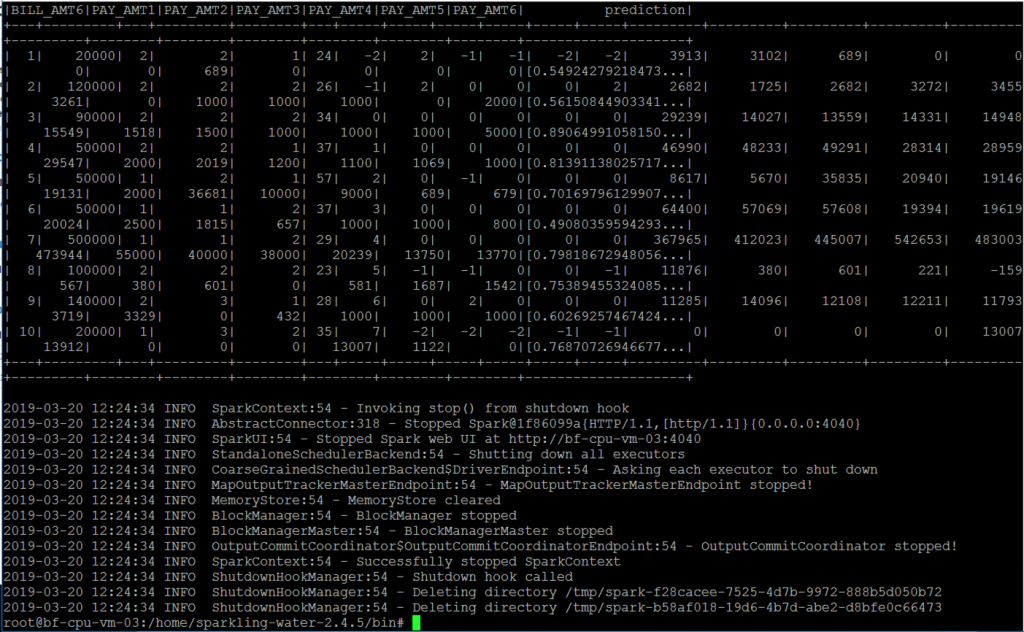
We can now examine the output data to see the results of the pipeline execution process, as shown in the “prediction” column (the rightmost one) of the output Spark DataFrame object. This test program used just 10 examples. For more extensive testing it can be run against larger datasets to generate more predictions. There are other methods of taking a MOJO pipeline to production, such as those using the MLleap framework, but those methods were not pursued as part of this exercise.

Conclusion

In this article, we see a method for executing a sanity test on a machine learning pipeline that is produced in MOJO format by the H2O Driverless AI tool. We then also see two separate methods of deploying that pipeline in a production environment, using the Java runtime and alternatively using standalone Apache Spark 2.4.0. The whole process, from the feature engineering, data analysis and model training, using H2O Driverless AI to the deployment steps taken here, is done using virtual machines on VMware vSphere as the platform. The process benefits from the isolation of versions and tools, hardware independence and flexibility of choice of tool and platform versions supported by the virtual machines and the underlying VMware vSphere hypervisor.

Appendix 1: Installation of Software in the Virtual Machines

For the guest operating system within the virtual machines used on vSphere, we used the Ubuntu 16.04  4.4.0-143-generic #169 x86_64 release

The host (physical) servers running these virtual machines were installed with VMware vSphere 6.7 update 1

The other installed software used in this article are listed below.

The OpenJdk Java JDK

To install the JDK on Ubuntu/Debian use the command: apt install openjdk-8-jdk

The Scala Language and Compiler version 2.12.8

Gradle 2.10 

Apache Spark 2.4.0

H2O Driverless AI

H2O Sparkling Water

H2O Driverless AI 1,5,4

We also concurrently used an earlier version of H2O Driverless AI (1.3.1) on a separate virtual machine for testing a model generated by different versions.

Appendix 2:  Using an H2O Sparkling Water External Cluster

There is an “internal” and “external” backend method for deploying H2O Sparkling Water. The external backend method has the advantage of separating the H2O components’ lifetimes from that of the Spark executors’ lifetimes, making it more robust in reacting to cluster changes – as described in the H2O documentation. The testing described here was done to try out the H2O Sparkling Water architecture on vSphere. You can consider this as an optional extra step that is an additional one to the production deployment process described above. An H2O Sparkling Water cluster deployment is not essential for deployment of an ML pipeline, though it can be used for that purpose. We show it here mainly for extra information, for those who may want to use Sparkling Water as an external backend. This architecture would be used mainly in the training and testing phases that would be driven in the H2O Flow tool, for example. This area is where Sparkling Water comes into its own as a backend process.

Set an environment variable as follows:

export H2O_EXTENDED_JAR=/home/sparkling-water-2.4.5/h2odriver-sw2.4.5-extended.jar

Then execute the command

java -jar $H2O_EXTENDED_JAR -name test -flatfile <path-to-flatfile>

a number of times (in our case, we did this twice for testing)  on the same or different VMs. This command brings up a Sparkling Water node per Java process on each machine. These Sparkling Water nodes broadcast to each other and become aware of their shared H2O cluster (or “H2O cloud”) independently. We see two example Sparkling Water nodes communicating with each other in the screen below.

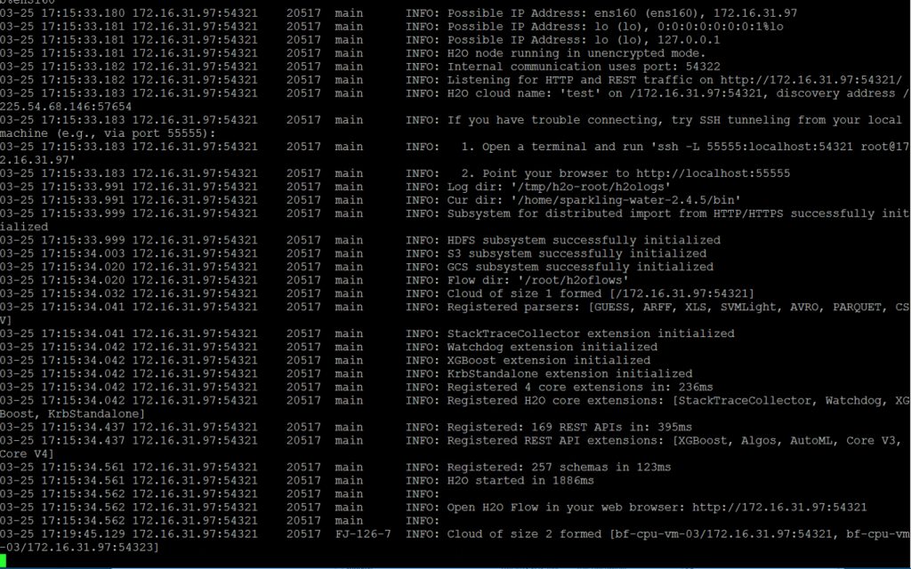
This “H2O Cloud” Sparkling Water cluster is set up to be independent of (external to) the Apache Spark cluster that we described above in our deployment setup, but it may be configured to inter-operate with that Apache Spark cluster, if need be. Connecting those two independent clusters would be done in order to make use of the complementary functionality of each cluster at different times (such as data munging in Spark, for example). We consider this topic as being out of scope for this article. For the purposes of this exercise, we want to confirm that we can bring up an “H2O Cloud” of Sparkling Water members and connect to it using the H2O Sparkling shell. The main advantage of Sparkling Water for our deployment is in the use of the Sparkling Water 2.4.5-assembly.jar file and its H2OMOJOModelPiepline class mentioned above.

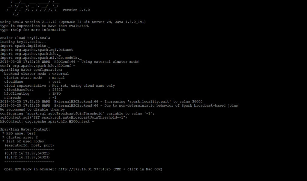
For validation of the functionality of our two-node H2O External cluster, we brought up a Sparkling-Shell process using the following commands

export JARS=license.sig,/opt/h2oai/dai/mojo2-runtime.jar,/home/sparkling-water-2.4.5/assembly/build/libs/sparkling-water-assembly_2.11-2.4.5-all.jar

$SPARKLING_WATER_HOME/bin/sparkling-shell

Within that Sparkling Water shell interface, we executed some straightforward checking commands, shown in code form below, that established an external cluster and accessed the H2OContext. We did not proceed with testing from there.