Co-author: Dave Jaffe, Staff Engineer
Many IoT systems such as those in manufacturing/testing facilities, connected cars and surveillance systems can generate huge quantities of data. Airplane engine testing, for example, can produce multiple gigabytes of measurement data per hour. Once all of that data is collected, the issue is making sense of it for monitoring and optimizing the particular business process or the behavior of the monitored device. This article discusses one method of exercising advanced analytics on the gathered data to achieve this optimization, using machine learning techniques.
The current article is based on an example set of applications that were written by VMware’s performance engineering personnel for the purposes of testing the Spark/MLlib application platform with VMware vSphere as the runtime environment. These tests were carried out on vSphere running on on-premises servers as well as on the VMware Cloud on AWS. The suite of programs ran unchanged on these environments. VMware Cloud on AWS runs the full set of vSphere Software Defined Data Center (SDDC) software, as the controlling software on sets of bare metal servers located at AWS data centers.
Using a new suite of Spark/MLlib-based programs, collectively called IoTStream, the end user can see the effects of different models, different quantities of data and different infrastructure for supporting the streaming data that flow from an instrumented IoT setup. This is useful as the back-end analysis phase of an overall IoT software suite. The motivation was to use machine learning techniques, starting with logistic regression, to help understand the behavior of incoming streamed data from the set of sensors, with the opportunity to scale that data up to measure performance. The details of running the suite, and of the amounts of data used in testing, are given below.
The high-level design of the IoTStream set of applications is shown in Figure 1.
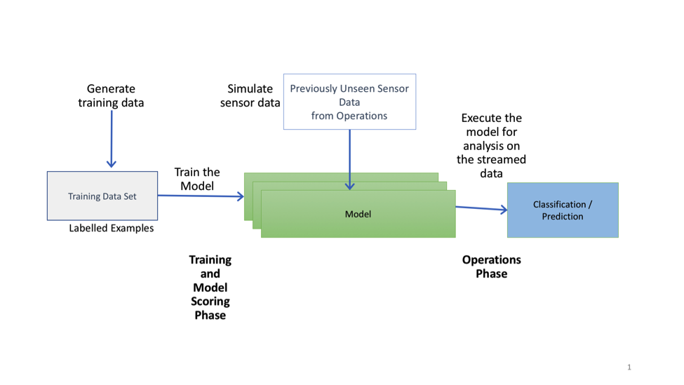
IoTStream: An IoT Application
Contents
IoTStream is a collection of Apache Spark-based programs that simulate the flow of data from an operation (such as a factory) with sensors generating data and the analysis of that data. The system continuously monitors the sensor values for fault conditions.
There are four different parts that make up the IoTStream suite. Those parts are as follows and are shown in figure 1:
(1) A Spark program that generates a set of synthetic training data with labels (iotgen);
(2) A Spark program that trains a machine learning model using that generated training data (iottrain);
(3) A Python script that generates testing/operational data. This data is kept separate from the training data and is designed to have values that are not found in the training data.
(4) A Spark program that uses the trained model in an operations context to detect potential failures in the testing data (iotstream).
These are run in the context of a Spark cluster that is started up before an execution begins. The Spark programs are invoked using the “spark-submit” commands shown in the figures below. The Spark Driver virtual machine uses a cluster of Spark workers (encapsulated in virtual machines) to execute the job of analyzing the data in a distributed fashion.
Using a Machine Learning Algorithm
The IoTStream analysis phase uses a machine learning model from the Spark MLlib library that is trained using the iottrain program mentioned above by applying the generated labelled data. We make a distinction between “training”, “testing” and “operational” data here – the training data has labels indicating good or bad records while the testing data has labels that are used for checking the accuracy of model prediction outputs only. The operational data does not contain these labels – those are the values that we want the model to predict. It is important to keep at least 30% of our overall data aside for testing after the model training has been carried out on 70% of our collected labeled data.
The labels in this machine learning training data indicate whether that particular example set of data (record) represents a good or bad set of sensor values. The IoTStream application, using the trained model, reads from a stream of operational data coming from the sensors and infers from its model whether the current set of sensor values indicates an imminent failure condition or not.
The particular machine learning algorithm applied in the sample application is a Logistic Regression, an example of the class of models called Generalized Linear Models. During the training of that model, several passes are made over the entire set of training data. This phenomenon, with multiple passes over the same data, is where the in-memory Resilient Distributed Dataset (RDD) functionality of Spark is particularly effective, compared to its predecessors.
A linear algebra mathematical model is constructed with weight values applied to each feature in the example data. The objective is to find those weight values that, when applied to the features of each example, provide a minimal difference between the output value of the equation and the known correct outcome, i.e. the label value. The technique applied to arrive at those weight values is called stochastic gradient descent or SGD. The difference between the output of the equation and the label value is the loss function and the goal is to find the weights that minimize the loss function. In that way, we know that our training is achieving a level of accuracy in the model’s predictions.
A useful analogy here is to imagine that you are situated at a high point in a hilly landscape, blindfolded, and that you want to take a step forward that will lead you toward the lowest point in the landscape. Training the model is the process of finding the right direction and size of step to take (the learning rate) so as to get to the bottom, the minimum difference, as efficiently as possible.
The logistic regression used here is a binary classifier that produces a positive or negative result when given a set of input data. Other classifiers are available in the machine learning libraries also.
The Infrastructure Setup
VMware Cloud on AWS
The deployment target for an application on VMware Cloud on AWS is a set of virtual machines that run on a unit called an SDDC (software-defined data center). You can think of the hardware component of an SDDC as one or more physical servers that live in an AWS data center location. Users and communities can construct many SDDCs, once they have a suitable account on VMware Cloud on AWS. Figure 2 shows a vCenter top-level view of the SDDC that we used for this set of two IoTStream applications.
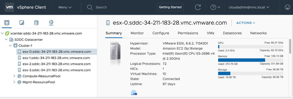
As you can see clearly in the vCenter interface, there were four physical servers in this example. There could be any number of physical servers present in an SDDC, depending on the needs. VMware configures these host servers during the SDDC provisioning process along with vSphere, vCenter, vSAN, VMware NSX and other components, without the user having to concern themselves with the details. From that point on VMware also manages the SDDC.
The SDDC physical host servers have the hardware specifications that can be seen in Figure 2. They also share a set of vSAN datastores that are used for the virtual machine files that are created by the user. These datastores are also pre-determined by VMware at SDDC provisioning time. In our testing, we used the datastore named “WorkloadDatastore” for all of our virtual machines. Here is the summary screen of the available datastores in our SDDC setup.

For our IoTStream application, we created four virtual machines on the above infrastructure, each with the configuration as shown in Figure 4 below. We had two instances of this setup for the IoTStream application set, each in a resource pool of its own (IOT1 and IOT2).
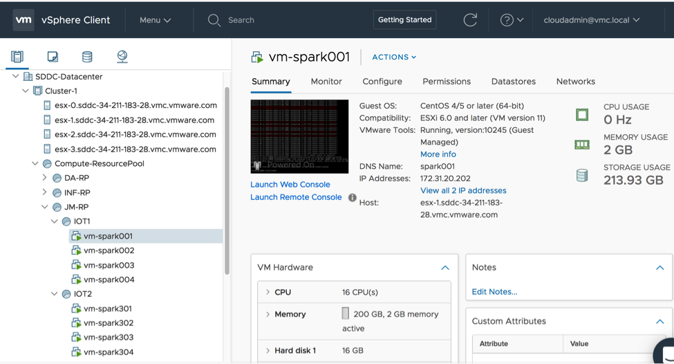
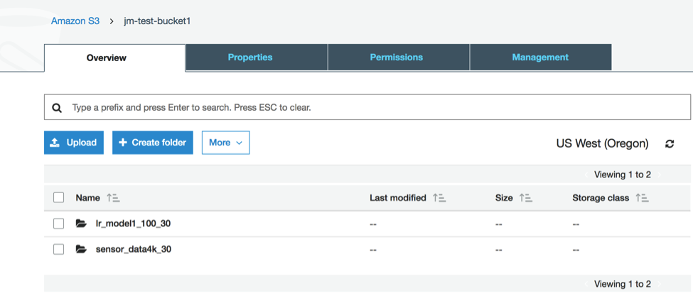
The virtual machines for the IoTStream application all had the same configuration. They each had 16 virtual CPUs, 200 GB of RAM and 16 GB of disk space on the WorkloadDatastore mentioned above. The training and model data that was created by the IoTStream application was held in S3 buckets that were outside of the vSAN datastores. These data items were accessed by the application code using “s3a://” URIs. The training data is shown in Figure 7 below, named as a “sensor_data4k_30”, object and the trained model are contained in the S3 object named “lr_model1_100_30”.
The vSAN datastores principally contained the VMDK and other related files to support the guest operating system. With this “separated” design, if a virtual machine needed to be moved from one host server to another using vMotion, then the application’s data on S3 was unaffected by that move. For the IoTStream application, a Hadoop Distributed File System (HDFS) facility is also available for storing the application/business data. This HDFS feature was used in the on-premises vSphere instance of the application.
Running the IoTStream Programs
The IoTStream application has four steps in it. Each step, apart from step 3, maps to a job that is executed on a Spark Driver virtual machine that itself is part of a running Spark cluster. The Spark cluster is started in the normal way before any of the IoTStream applications are run. The Spark Driver virtual machine uses a cluster of Spark workers (encapsulated in virtual machines) to execute the job of analyzing the data in a distributed fashion.
The commands to be executed to start the Spark cluster from the spark001 virtual machine’s command line are:
|
$SPARK_HOME/sbin/start–master.sh $SPARK_HOME/sbin/start–slaves.sh |
This latter command does a remote login to each virtual machine mentioned in $SPARK_HOME/conf/slaves on the spark001 VM and executes a script there to get that slave VM to connect to the cluster)
Once the Spark cluster is operating correctly, then using the Spark Driver virtual machine, the following steps are executed:
Generate sample sensor data (training data)
This step executes the “iotgen” Scala program. The program generates synthetic training data using a simple randomized model. Each row of the sensor data is preceded by a label whose values are 0 or 1. The 1 value in the label indicates that the set of corresponding feature values would trigger the failure condition, while the 0 value indicates that the associated feature values would not (normal state). The “iotgen” program generates and writes the training data either to an HDFS file or to a file within a unique S3 bucket. Here is a view of a single test run of this part.

Train a machine learning model using that data
The machine learning model (such as a Logistic Regression algorithm from MLlib) is trained on the generated data from step 1. Once the training has been completed, the trained model itself is then saved to an object in the HDFS file or a file in the named S3 bucket. Here is an image of the command to execute this part.

Once the generated data has been created and the logistic regression model is trained, you can view the outputs of each step in the AWS console for S3. You should see output similar to the following:
Simulate new test sensor data (as would occur in an operations context)
A Python script creates a stream of new sensor data at a certain interval, as follows:

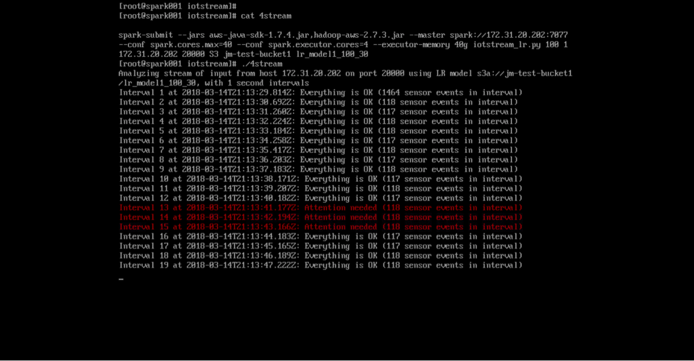
Execute a test sequence
The goal is to read the streamed sensor data and make decisions about it using the machine learning model – checking whether the sensor data indicates that a fault condition is occurring or about to occur or not.
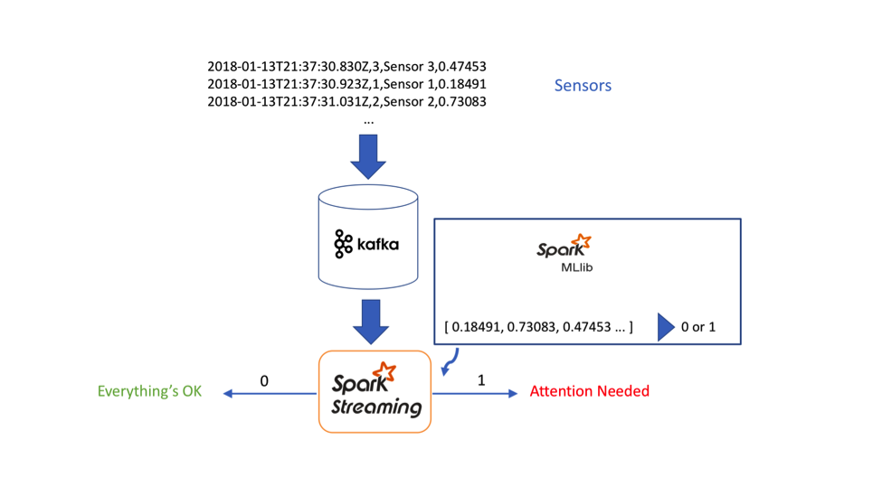
The IoTStream application is designed such that communication of the sensor data between the components can be done over a TCP/IP socket or alternatively over Kafka, for highly resilient messaging. Figure 10 shows the data flow from the sensors to the model operating over Kafka.
Observations
We can naturally run two or more parallel copies of this application on the same virtualized infrastructure. To do this, there are two instances of IoTStream running in parallel in two separate sets of virtual machines hosted in separate resource pools on VMware Cloud on AWS. We separate the output files from the first two stages within the set of programs by using a separate destination S3 bucket or HDFS destination.

One of these IoTStream application clusters can be used for development, while the other would be a pre-production staging or a production cluster. This type of setup is shown in conceptual form in Figure 12.
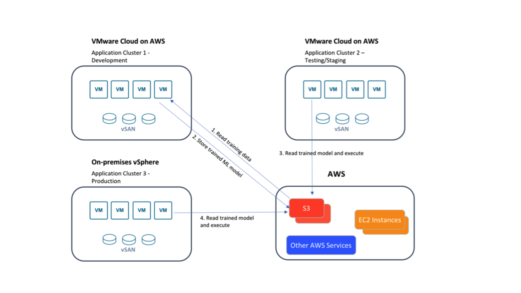
We can train a model in one cluster (e.g. cluster 1, with training data) and then use it for testing in another, (cluster 2, with testing data) leaving a data scientist to carry on refinement in the first one while we are executing the original version elsewhere.
Furthermore, since we are using public cloud storage (S3) to store the trained model itself, we can then use that trained model artifact in either the public cloud analysis or in an on-premises analysis. Parts of our application are now potentially in both environments, but operating independently of each other. We used this approach in our test lab to move models between different clusters. Training may best be done for large data sets in the public cloud, whereas execution of the resulting model from that training can be done on-premises, where the production data originated. A data science department would incorporate this facility into their CI/CD pipeline.
Benchmarking
As a benchmark, iotgen is an excellent I/O test, taking on the order of 10 minutes to generate 1TB of data (8M rows with 10,000 sensor points each) on an on-premises 10-server Spark cluster. The iottrain program took about 20 minutes to train a model with that data on the same cluster. IoTStream has been tested with up to 100,000 sensor events per second on a single virtual machine.
Conclusions
In this article, we show a collection of Spark-based programs running unchanged across vSphere on-premises and on VMware Cloud on AWS. The programs act together to train a machine learning model on one set of IoT data and then make predictions or decisions about new, unseen examples of the same type of data when presented with it over Spark streaming mechanisms.
The ML model could be trained in a public cloud-hosted cluster and then used in a private cloud one, or vice versa. Models can be re-trained offline from their inference execution in different clusters or implementations. This allows us to improve the model with new training data or change it out completely while executing an older version elsewhere. This sample suite of programs on Spark shows the power and flexibility of virtualization and VMware Cloud on AWS for deployment of IoT analysis and machine learning systems such as this one.
Co-author: Dave Jaffe, Staff Engineer

